IB Biology · Theme C · C4.1

Populations and communities

From counting a handful of quadrats to explaining a decade-long lynx-and-hare cycle, this lesson follows populations from a single defining trait — members that interbreed — through the maths of growth and the negative feedback that keeps it in check, into the full cast of relationships, tests and controls that shape a real community.

Guiding questions

How do interactions between organisms regulate sizes of populations in a community?

What interactions within a community make its populations interdependent?

Part one

Measuring populations

C4.1.1 – C4.1.4

C4.1.1

One species, one breeding group

A population is a group of interacting organisms of the same species living in the same area at the same time, whose members normally breed with one another.

Two groups of the same species are treated as separate populations when a barrier — distance, a mountain range, an unconnected lake — normally prevents individuals from interbreeding.
This reproductive isolation, not physical differences in size or appearance, is the defining test used to distinguish one population from another.
If the barrier disappeared, the two groups would simply become one population again — separation alone does not create a new species.

Why it mattersA population is not just "organisms in an area" — that fits a community; a population is specifically one interbreeding species.

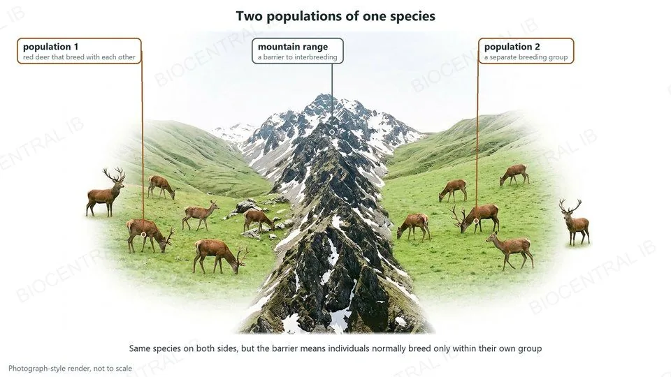
Photograph-style render of red deer grazing in two valleys separated by a mountain range: two populations of one species, because the barrier means individuals normally breed only within their own group

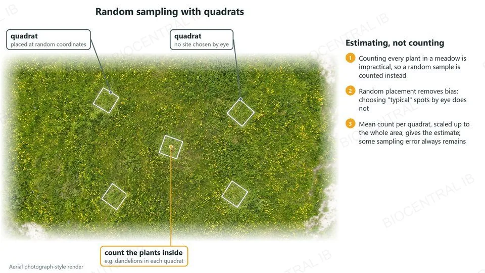
Aerial photograph-style render of a meadow with dandelions and five square quadrats placed at random coordinates; the plants inside each quadrat are counted and the mean is scaled up to the whole area

C4.1.2

Why sample instead of count

Ecologists estimate population size by random sampling rather than counting every individual, because a complete census of most natural populations is impractical or impossible.

Individuals may be numerous, mobile, hidden, or spread across a large or inaccessible area — sampling a representative subset and extrapolating gives a workable estimate at far lower cost.
Sampling must be random: if a researcher subjectively picks "typical-looking" or convenient sites, the estimate becomes systematically biased rather than just imprecise.
Even perfectly random sampling still leaves sampling error — an unavoidable difference between the estimate and the true population size, distinct from bias.

Why it mattersRandom sampling removes systematic bias; it does not, and cannot, eliminate sampling error altogether.

C4.1.3

A frame, randomly placed

Random quadrat sampling estimates population size for sessile organisms — plants, and animals fixed in place such as barnacles — by counting individuals inside a fixed sample area placed at random positions.

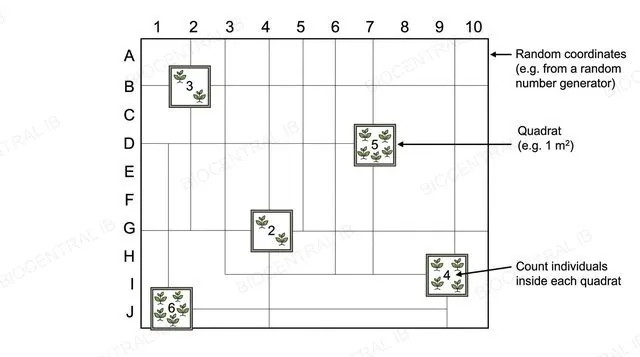
Quadrat positions are set using random coordinates, for example from a random number generator over a grid — never chosen because a spot "looks representative," which reintroduces bias.
The method only works if individuals stay within the quadrat long enough to be counted, which is why it suits sessile organisms rather than motile animals.
The mean count per quadrat gives the density; multiplying it by the number of quadrat-sized areas in the study area (total area ÷ quadrat area) estimates the population size.

Why it mattersQuadrats are not a general-purpose method for any organism — their validity depends entirely on the organism staying still long enough to count.

A flat diagram of a numbered and lettered grid over a field with five small quadrat frames placed at random coordinates, each containing a counted number of plant icons, labeled random coordinates and quadrat 1 square metre

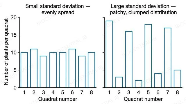
A flat two-panel bar chart with numeric y-axis values for number of plants per quadrat, left panel showing eight similar-height bars labeled small standard deviation evenly spread, right panel showing eight wildly varying bars labeled large standard deviation patchy clumped distribution

C4.1.3 · Skills

What the spread is telling you

The standard deviation of the mean number of individuals per quadrat measures how evenly a population is spread across the sampled area — students are not expected to memorise its formula, only to interpret it.

A small standard deviation means quadrat counts cluster close to the mean — the population is distributed fairly evenly across the field.
A large standard deviation means counts vary widely between quadrats — the population is patchy or clumped rather than evenly spread.
Standard deviation says nothing about population size itself — a large or a small total population can each show either a small or a large spread.

Why it mattersConfusing "spread across the area" with "size of the population" is the most common misreading of this statistic.

C4.1.3 · Data booklet

The booklet’s normal curve shows what SD means

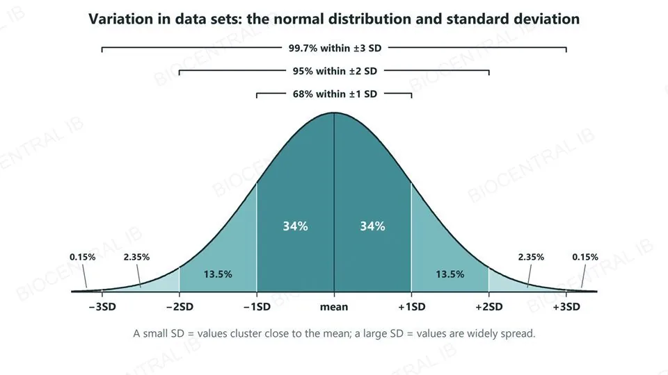
For data that follow a normal distribution, the data booklet shows how values spread around the mean in units of standard deviation (SD).

About 68% of values lie within 1 SD of the mean, 95% within 2 SD and 99.7% within 3 SD.
On each side of the mean: 34% lie between the mean and 1 SD, 13.5% between 1 and 2 SD, 2.35% between 2 and 3 SD, and 0.15% beyond 3 SD.
Example: a mean of 12 plants per quadrat with an SD of 2 means about 68% of quadrats hold 10–14 plants.

Why it mattersThe curve and its percentages are in the data booklet — you need to interpret SD, not memorise it.

A normal distribution curve divided at the mean and at 1, 2 and 3 standard deviations either side, with 34%, 13.5%, 2.35% and 0.15% of values in each band, and brackets showing 68% within 1 SD, 95% within 2 SD and 99.7% within 3 SD of the mean

C4.1.4 · Skills

Marking a sample, twice

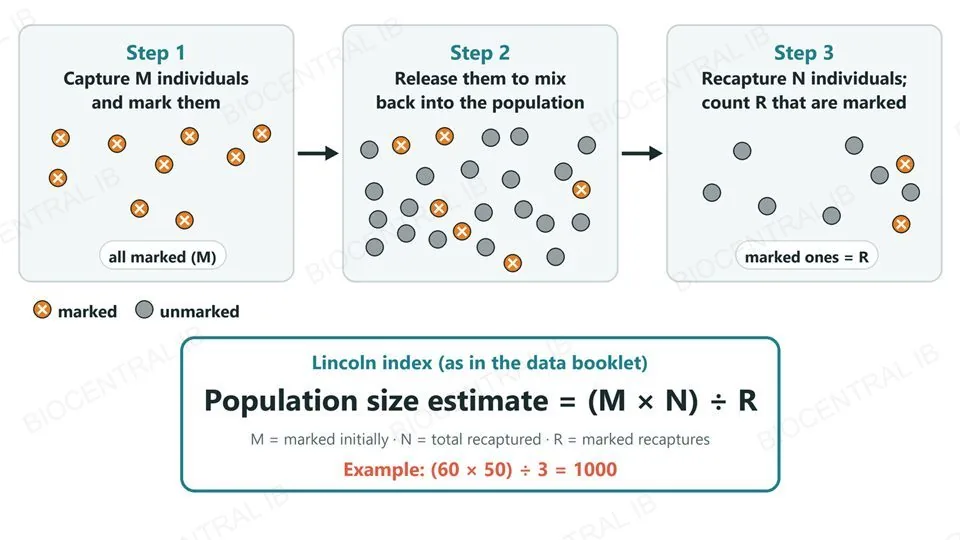
Capture-mark-release-recapture estimates population size for motile organisms using the Lincoln index, written in the data booklet as: population size estimate = (M × N) ÷ R.

A first sample of M individuals is caught, marked without affecting survival, and released to mix randomly back into the population.
A second sample of N individuals is caught later; the marked proportion of that sample (R out of N) is assumed to match the marked proportion of the whole population (M out of the total).
Rearranging gives population size = (M × N) ÷ R; for example, 60 marked, 50 recaptured and 3 of them marked gives (60 × 50) ÷ 3 = 1,000.

Why it mattersWatch the letters: in the data booklet N is the total recaptured, not the population — the population size is what you calculate.

Three panels: step 1, capture M individuals and mark them; step 2, release them to mix back into the population; step 3, recapture N individuals and count R that are marked. Below, the Lincoln index as written in the data booklet: population size estimate equals M times N divided by R, with the example 60 times 50 divided by 3 equals 1000.

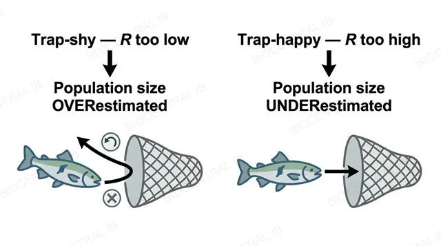
A flat two-panel diagram, left panel labeled trap-shy R too low leading to population size overestimated, right panel labeled trap-happy R too high leading to population size underestimated

C4.1.4 · Skills

When the assumptions break

The Lincoln index is only valid if marked individuals mix randomly, marks are not lost, catching is random, and the population is closed — no significant births, deaths, immigration or emigration between samples.

If marked individuals become "trap-shy" and avoid recapture, R is artificially low — since R sits in the denominator, this inflates the estimate, overestimating the population.
If marked individuals become "trap-happy" and are recaptured more easily, R is artificially high, deflating the estimate and underestimating the population.
The direction of the error can be deduced from which of M, N or R is affected — not just labelled "wrong."

Why it mattersSaying which direction an estimate is skewed, and why, shows real understanding rather than just quoting the formula.

Quick check

A researcher marks and releases 60 crabs. Two days later she catches 50, but only 3 are marked, because marked crabs avoid her traps. What effect does this have on her Lincoln index estimate?

No effect — trap-shyness does not change the calculation

The population size will be overestimated, because R (marked recaptures) is artificially low

The population size will be underestimated, because R is artificially high

The estimate becomes impossible to calculate

Correct answer: overestimated. Population size estimate = (M × N) ÷ R = (60 × 50) ÷ 3 = 1,000 — R is in the denominator, so trap-shy behaviour lowering R inflates the estimate, making the population look larger than it really is.

Part two

Population growth

C4.1.5 – C4.1.8

C4.1.5

The ceiling an environment sets

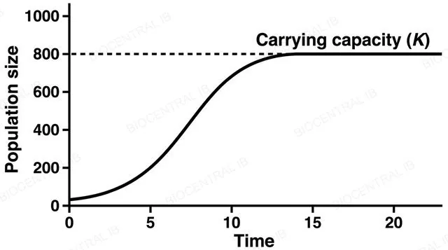
Carrying capacity (K) is the maximum population size that an environment can sustain, set by whichever resource — food, water, space, nesting sites — runs out first.

Below K, there are enough resources per individual for the population to keep growing; at K, growth levels off because the limiting resource is fully used.
K is not a fixed number for a species — it depends on the specific environment, and can rise or fall as resource availability changes, for example with drought, rainfall, or habitat destruction.
As a population nears K, competition for the limiting resource intensifies between individuals of that same species.

Why it mattersTreating K as a permanent property of a species, rather than of a species-in-an-environment, is a common and testable misconception.

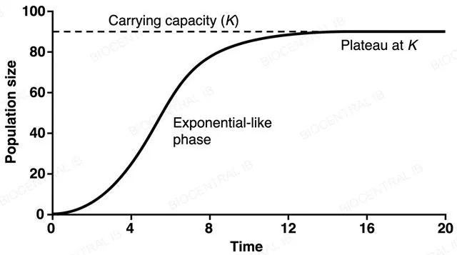
A flat line graph with numeric axes showing population size rising then flattening into a plateau, with a horizontal dashed line labeled carrying capacity K marking the plateau level

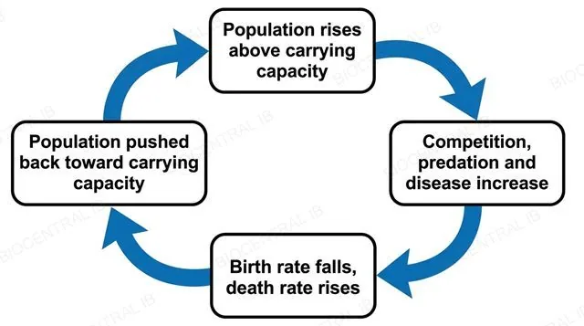
A flat circular feedback loop diagram with four boxes connected by same-direction arrows: population rises above carrying capacity, competition predation and disease increase, birth rate falls and death rate rises, population pushed back toward carrying capacity, looping back to the first box

C4.1.6

Pulled back toward the ceiling

Density-dependent factors push a population back toward carrying capacity through negative feedback, with their effect intensifying as population density rises.

As density increases, competition for limited resources, the risk of predation, and the transfer of pathogens or pests between individuals all become more severe.
These pressures lower the birth rate and raise the death rate, slowing growth and pushing the population back toward K — a self-correcting, negative-feedback response.
Density-independent factors, such as a storm or a wildfire, also cause fluctuations, but their impact does not depend on how crowded the population already is.

Why it matters"Density-independent" means the impact doesn't scale with density — not that the factor has no effect on the population at all.

C4.1.7

Growth with nothing in the way

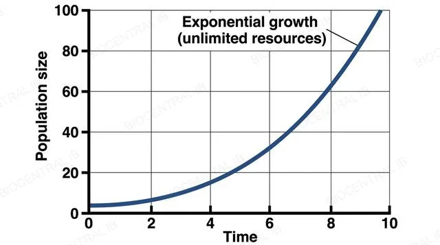
Exponential growth occurs when resources are effectively unlimited relative to population size, so the population grows at a constant per-capita rate, producing a J-shaped curve.

This typically happens in the initial phase of colonising a new environment, while numbers are still small enough that competition for resources is negligible.
Real populations almost never sustain exponential growth for long — as numbers rise, density-dependent factors increasingly slow growth, and the idealised J-shaped curve is a simplification, not a literal prediction.
This nature-of-science point matters generally: models like this curve are useful precisely because they simplify a genuinely more complex real system.

Case studyIn 1911, 25 reindeer were released on St Paul Island, Alaska. With plenty of lichen and no predators they grew almost exponentially, to about 2,000 by 1938, before overgrazing crashed the herd.

A flat line graph with numeric axes showing a single upward curving J-shaped exponential growth curve rising steeply from time zero with no plateau and no flat starting phase, labeled exponential growth unlimited resources

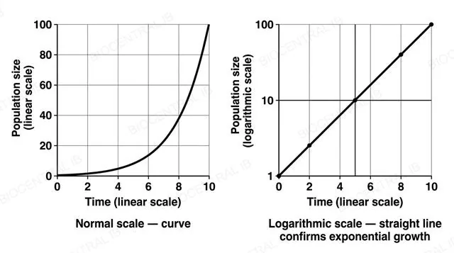
A flat two-panel diagram with numeric axes, left panel a normal-scale graph showing a steeply curving exponential line labeled normal scale curve, right panel a logarithmic-scale graph showing a perfectly straight diagonal line labeled logarithmic scale straight line confirms exponential growth

C4.1.7 · Skills

Turning a curve into a line

Whether a population is truly growing exponentially can be tested by plotting population size on a logarithmic scale against time on a normal, linear scale.

Exponential growth follows N = N₀e^(rt); taking the logarithm of both sides gives a straight-line relationship between log(N) and time.
On an ordinary linear-linear graph, exponential growth is a curve that gets steadily steeper, which is hard to distinguish confidently from other fast-growth patterns by eye.
On the log-linear plot, genuine exponential growth appears as a straight line — any curvature away from a straight line shows the growth is departing from the exponential model.

Why it mattersThis turns a subjective "does this curve look exponential?" judgement into an objective straight-line test.

C4.1.8 · Skills

Growth that curves over

The sigmoid (S-shaped) population growth curve models growth that speeds up, slows down and then levels off at carrying capacity — in this idealised model, a flat lag phase is not expected at the start.

Growth is close to exponential at first and fastest at about half of K, then slows as density-dependent factors take effect, and levels off at K.
Yeast and duckweed are the recommended organisms for collecting real growth data — both proliferate rapidly under simple conditions and can be counted repeatedly.
Real experimental data, unlike this idealised model, often does show an initial lag — a reminder the curve is a simplification, not a perfect real-world description.

Why it mattersDrawing a flat lag segment onto the idealised sigmoid curve itself is a specific, avoidable error.

A flat line graph with numeric axes showing an S-shaped sigmoid curve rising immediately from time zero with no flat lag segment, curving through a steep middle phase, then flattening into a plateau at a horizontal dashed line labeled carrying capacity K

Quick check

The idealised sigmoid growth curve rises immediately from time zero with no flat lag segment, but a real yeast culture in a flask often shows a genuine flat lag phase before growth speeds up. What does this contrast best illustrate?

The sigmoid model is wrong and should be abandoned

Real yeast populations never actually follow a sigmoid pattern

The sigmoid curve is an idealised graphical model — a simplification that can still leave out features, like a lag phase, seen in real data

Carrying capacity does not apply to yeast populations

Correct answer: models are simplifications. Both the exponential and sigmoid curves are idealised graphical models; real populations can show extra features, such as an initial lag phase, that the simplified model does not include.

Part three

Communities and interactions

C4.1.9 – C4.1.18

C4.1.9

Same species, two outcomes

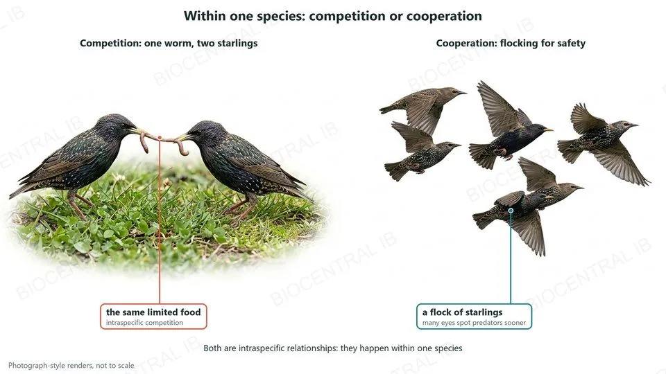
Individuals of the same species can either compete for limited resources or cooperate for mutual benefit — both are intraspecific relationships, since they occur within one species.

Intraspecific competition arises because members of a species need the same resources — food, light, space, mates — so it is often intense; densely sown seedlings, for example, compete for light and grow smaller.
Intraspecific cooperation can raise the survival or reproductive success of the group: wolves hunt in packs, meerkats take turns as sentries, and worker honeybees raise the colony's young.
Whether competition or cooperation dominates in a given population depends on the specific resource and behaviour involved, not a fixed rule for the species.

Why it matters"Intraspecific" specifically means within one species — this is what separates it from every interspecific relationship covered next.

Photograph-style renders of starlings: two starlings pulling at the same worm, intraspecific competition for limited food; and a flock of starlings flying together, cooperation in which many eyes spot predators sooner

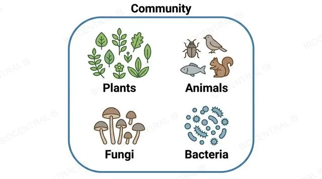
A flat diagram of one large rounded boundary labeled community containing four labeled clusters of icons: plants, animals, fungi, and bacteria

C4.1.10

Every population, together

A community is all of the interacting populations of different species living in an area — plants, animals, fungi and bacteria alike.

A community is broader than a population, which is only one species, but narrower than an ecosystem, which also includes the abiotic environment such as soil, water and climate.
Members of a community interact through the whole range of relationships covered in this topic — feeding, competing, and cooperating across species.
A pond community, for example, includes its fish, plants, algae and bacteria, but not the water or dissolved oxygen those organisms live in.

Why it mattersMixing up population, community and ecosystem is one of the most common vocabulary errors in this entire topic.

C4.1.11

Consumer relationships, three ways

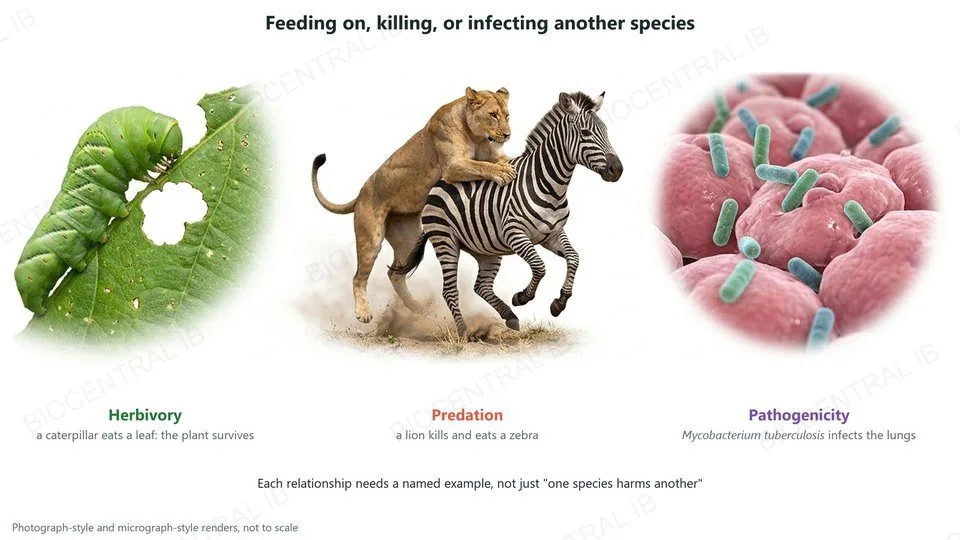
Herbivory, predation and pathogenicity are three categories of interspecific relationship in which one species feeds on, kills, or causes disease in another.

Herbivory is an animal feeding on a plant, such as a caterpillar eating a leaf — the plant is typically damaged but not killed outright.
Predation is one animal killing and eating another, such as a lion killing a zebra — a direct, usually fatal, consumer-resource interaction.
Pathogenicity is a pathogen (a virus, bacterium, fungus or protist) causing disease in a host, such as the bacterium Mycobacterium tuberculosis causing tuberculosis in humans.

Why it mattersEach category needs at least one specific, nameable example — a vague description of "one species harming another" is not enough on its own.

Photograph-style and micrograph-style renders: a caterpillar eating a leaf, herbivory, in which the plant survives; a lion bringing down a zebra, predation; and rod-shaped Mycobacterium tuberculosis bacteria on lung cells, pathogenicity

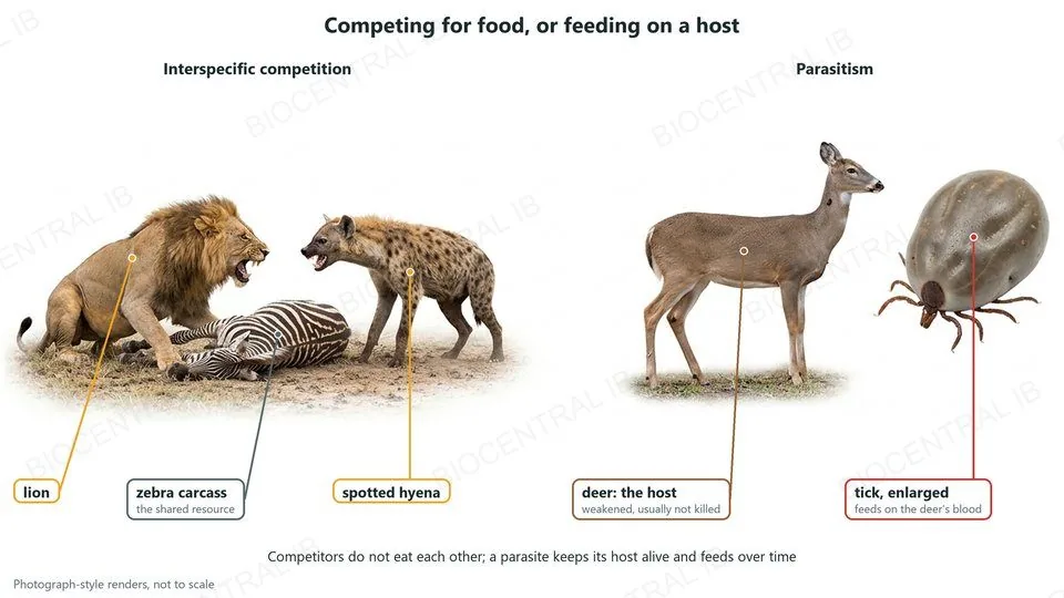
Photograph-style renders: a lion and a spotted hyena competing over a zebra carcass, interspecific competition; and a deer with an enlarged tick that feeds on its blood, parasitism, in which the host is weakened but usually not killed

C4.1.11

Sharing, and taking slowly

Interspecific competition and parasitism are two more categories of interspecific relationship; the sixth, mutualism, follows next.

Interspecific competition occurs when different species compete for the same limited resource, such as lions and hyenas competing for the same prey — neither directly consumes the other.
Parasitism is one species living on or in a host and feeding from it over time, weakening but usually not killing it, such as a tick feeding on a deer.
Distinguishing the two matters: a parasite typically keeps its host alive, since a dead host is no longer a food source.

Why it mattersMatching each relationship name to the correct real-world example — not just recognising the surface topic — is the actual skill being tested.

C4.1.12

When both sides gain

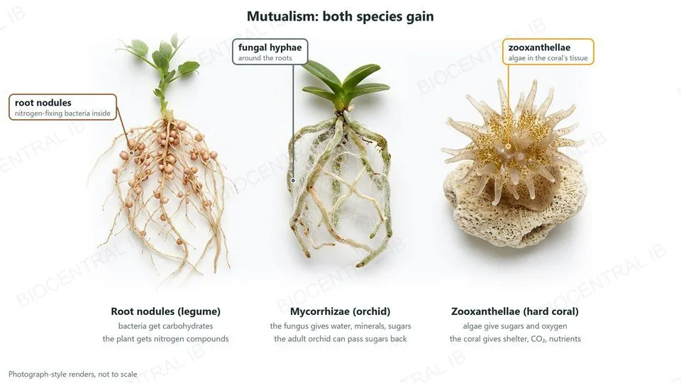
Mutualism is an interspecific relationship that benefits both species involved, illustrated here by three required examples: root nodules, mycorrhizae, and zooxanthellae.

Root nodules in legumes (Fabaceae) house nitrogen-fixing bacteria: the bacteria receive carbohydrates from the plant, and the plant receives usable nitrogen it could not otherwise obtain from the air.
Mycorrhizae in orchids (Orchidaceae): the fungus supplies water and minerals such as phosphate; orchid seeds have almost no food store, so the fungus also feeds the seedling sugars, and the green adult orchid can pass sugars back.
Zooxanthellae are photosynthetic algae living inside hard coral tissue, supplying the coral with sugars and oxygen in exchange for shelter, carbon dioxide and nutrients from the coral's waste.

Why it mattersMutualism is an exchange, not altruism — naming the specific benefit each partner receives is what full marks require.

Photograph-style renders of three mutualisms: legume roots with nodules holding nitrogen-fixing bacteria; an orchid seedling whose roots are wrapped in fungal hyphae, mycorrhizae; and a hard coral polyp whose tissue holds zooxanthellae algae

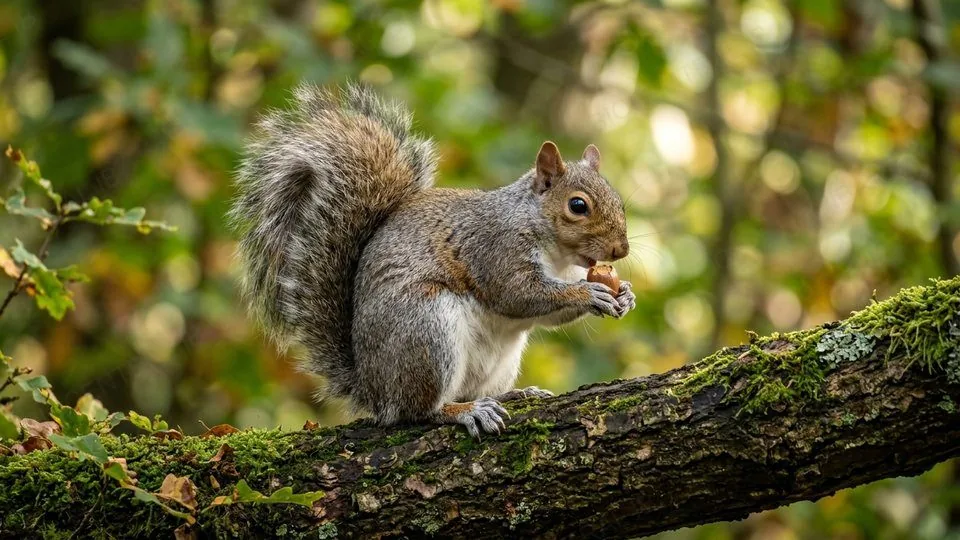
An eastern grey squirrel sitting on a mossy branch, eating an acorn held in its front paws; grey squirrels were introduced to Britain from North America

C4.1.13

More food from the same trees

Resource competition between an endemic and an invasive species can give the invader a competitive advantage in acquiring resources, which is one basis for it becoming invasive.

Grey squirrels, introduced to Britain from North America in the late 1800s, compete with the native red squirrel for the same tree seeds.
Greys digest acorns, which are rich in tannins, far better than reds can, so in broadleaf woodland they get more food from the same trees — and they also raid the reds' buried seed stores.
Red squirrels have disappeared from most of England and Wales where greys spread; a squirrelpox virus carried by greys adds to the decline.

Why it mattersThe guide asks for one local example: if your region has its own invasive competitor, learn it the same way — which resource, and why the invader gets more of it.

C4.1.14 · NOS

Suggestive is not proof

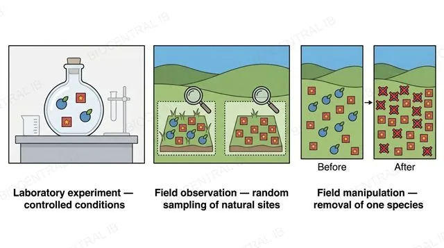
Interspecific competition is indicated, but not proven, if one species is more successful in the absence of another — three research approaches can test for it more rigorously.

Laboratory experiments grow two species together and separately under controlled conditions, isolating competition from other variables.
Field observations use random sampling to compare sites where both species occur against sites where only one does, looking for a consistent pattern.
Field manipulation removes one species from a plot and compares the other species with an untouched control plot — when Connell removed Balanus barnacles from Scottish rocks, Chthamalus survived lower on the shore.

Why it mattersRecognising the difference between an experiment (a variable is manipulated) and an observation (patterns are recorded without intervention) is a specific nature-of-science skill here.

A flat three-panel diagram: a sealed container with two species on a lab bench labeled laboratory experiment controlled conditions, a landscape with two sites compared under a magnifying glass labeled field observation random sampling, a field shown before and after one species is removed labeled field manipulation removal of one species

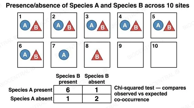
A flat diagram of a grid of ten sampling sites showing presence or absence of Species A and Species B, with a two by two table of observed counts six one one two, labeled chi-squared test compares observed versus expected co-occurrence

C4.1.15 · Skills

Testing whether two species avoid each other

A chi-squared test can be applied to the presence or absence of two species across several sampling sites, exploring whether their distributions are associated.

Each site is recorded as having both species present, only one, or neither, building an observed-frequency table like the one shown.
The chi-squared test compares these observed counts with the counts expected if the two species were distributed completely independently of each other.
A significant difference shows the two species are associated: found together less often than expected (possible evidence of competition) or more often (for example, shared habitat needs).

Why it mattersThis gives the "one species more successful in the absence of another" idea from the previous statement an actual statistical test.

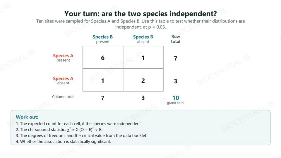
A two by two observed-value table for Species A present or absent against Species B present or absent, with row, column and grand totals, followed by a four-item to-do list: find the expected values, calculate chi-squared, find the degrees of freedom and critical value, and decide on significance.

C4.1.15 · Skills · Try it yourself

Before the answer: try the test yourself

The same ten-site presence/absence data from the previous slide, set as a task rather than a worked answer.

Find the expected value for each of the four cells, assuming the two species are distributed independently of each other.
Calculate the chi-squared statistic, work out the degrees of freedom, and look up the critical value in the data booklet.
Decide whether the observed pattern is statistically significant at p = 0.05, or could plausibly be due to chance.

Why it mattersWorking the whole test yourself, before seeing it solved, is what actually builds the skill the exam tests.

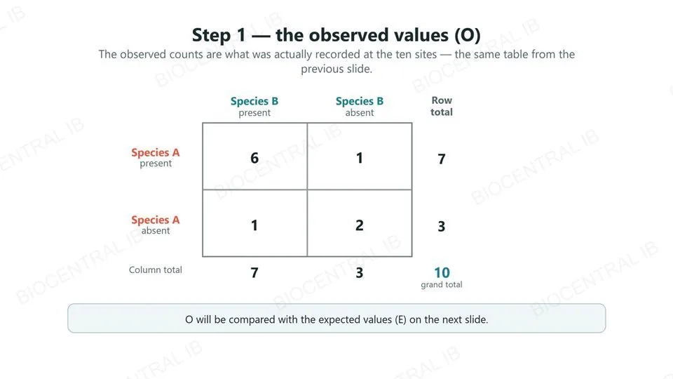
A two by two table of observed counts, six one one two, with row totals 7 and 3, column totals 7 and 3, and a grand total of 10.

C4.1.15 · Skills · Worked example, step 1

Step 1 — lay out the observed values

The first step of any chi-squared test is a clear table of what was actually counted.

Six sites had both species, one had only Species A, one had only Species B, and two sites had neither.
Row totals (7 and 3) and column totals (7 and 3) both add up to the grand total of 10 sites.
Hypotheses: H₀ — the two species are distributed independently (no association); H₁ — their distributions are associated.

Why it mattersEvery later step in the test starts from this one table, so it has to be right before anything else is calculated.

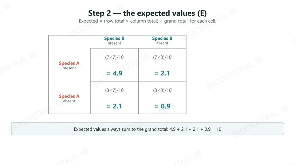
The same two by two table with each cell showing its expected-value formula, row total times column total divided by grand total, and the result: 4.9, 2.1, 2.1 and 0.9.

C4.1.15 · Skills · Worked example, step 2

Step 2 — calculate the expected values

The expected value for a cell is what its count would be if the two species were completely independent.

Expected = (row total × column total) ÷ grand total, calculated separately for each of the four cells.
The four expected values are 4.9, 2.1, 2.1 and 0.9 — and, like the observed values, they also sum to 10.
Expected values do not have to be whole numbers: they describe an average outcome, not a possible single count.

Why it mattersChi-squared measures how far the real counts (O) are from this no-association baseline (E).

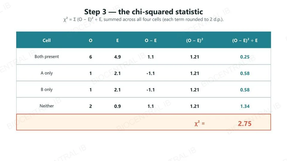
A six-column table listing each cell, its observed and expected value, O minus E, (O minus E) squared, and (O minus E) squared divided by E, with a highlighted total row reading chi-squared equals 2.75.

C4.1.15 · Skills · Worked example, step 3

Step 3 — work out chi-squared

The chi-squared statistic sums a standardised difference between observed and expected for every cell.

For each cell, calculate (O − E)² ÷ E — squaring removes the sign, and dividing by E scales it to that cell’s size.
The four terms are 0.25, 0.58, 0.58 and 1.34.
Summed across all four cells, χ² = 2.75.

Why it mattersA single combined number makes it possible to compare the whole table against one critical value, rather than judging four differences separately.

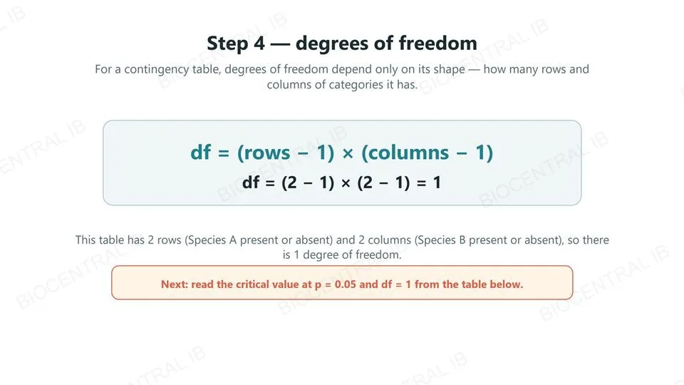
The formula degrees of freedom equals rows minus one times columns minus one, applied to a two by two table to give one degree of freedom.

C4.1.15 · Skills · Worked example, step 4

Step 4 — find the degrees of freedom

Degrees of freedom set which column of the critical-value table applies, and depend only on the table’s shape.

For a contingency table: degrees of freedom = (number of rows − 1) × (number of columns − 1).
This table has 2 rows (Species A present or absent) and 2 columns (Species B present or absent).
df = (2 − 1) × (2 − 1) = 1.

Why it mattersThe degrees of freedom, not the number of sites sampled, is what selects the correct column of the critical-value table.

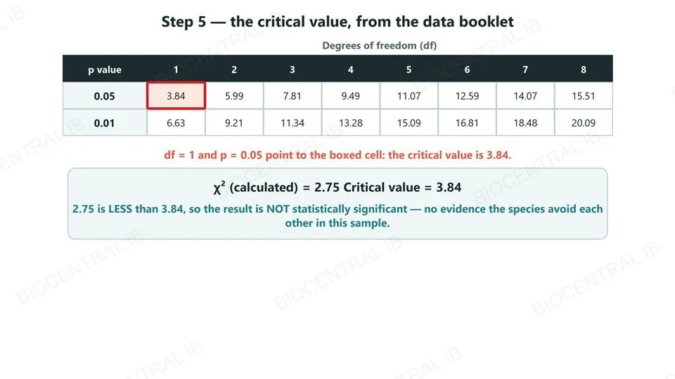
The data booklet’s chi-squared table, degrees of freedom 1 to 8 across the top and p values 0.05 and 0.01 down the side, with the cell at df 1 and p 0.05 boxed in red showing 3.84, followed by a summary comparing the calculated chi-squared of 2.75 with the critical value of 3.84 and concluding the result is not significant.

C4.1.15 · Skills · Worked example, step 5

Step 5 — compare with the critical value

The last step reads a threshold off the data booklet’s chi-squared table and compares it with the calculated statistic.

In the data booklet’s chi-squared table, the row p = 0.05 and the column df = 1 meet at the boxed cell: 3.84.
The calculated χ² (2.75) is less than the critical value (3.84).
Because 2.75 is smaller, H₀ is not rejected: there is no significant association between the two species at p = 0.05.

Why it mattersA χ² below the critical value means the observed pattern is within the range chance alone could produce — a real study would need a larger sample before concluding either way.

C4.1.16

A cycle that lags behind

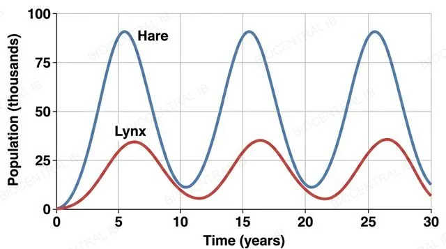
Predator-prey relationships are a real case study of density-dependent control: Canada lynx and snowshoe hare populations, tracked for over a century through Canadian fur-trapping records, cycle together roughly every ten years but out of phase.

When hares are abundant, lynx have more food, so kitten survival rises — but this takes time, so the lynx peak lags roughly one to two years behind the hare peak.
Rising predation, combined with the hares' own food shortage at high density, then crashes the hare population.
With less food available, the lynx population crashes too, releasing pressure on the hares and letting the cycle begin again.

Why it mattersThe defining feature of this cycle is the time lag — predators never track prey numbers instantly.

A flat line graph with numeric axes showing two oscillating population curves over time, a high-amplitude hare curve and a lower-amplitude lynx curve whose peaks visibly lag behind the hare curve's peaks

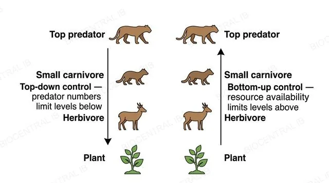
A flat two-panel vertical food chain diagram, left panel showing a downward arrow from a top predator through all trophic levels labeled top-down control predator numbers limit levels below, right panel showing an upward arrow from a producer through all trophic levels labeled bottom-up control resource availability limits levels above

C4.1.17

Control from above, or from below

Populations can be controlled top-down, by predator numbers limiting the levels beneath, or bottom-up, by resource availability limiting the levels above — both are possible, though usually one dominates.

Top-down: a change in predator numbers cascades downward. A widely cited case: after wolves returned to Yellowstone in 1995, elk browsing fell and streamside willows recovered in places.
Bottom-up: a change in resources cascades upward. In El Niño years the nutrient-rich upwelling off Peru weakens, phytoplankton decline, and anchovies and the seabirds that eat them crash.
Identifying which dominates in a real community usually needs evidence from an actual change at one trophic level and its knock-on effects.

Why it mattersBoth kinds of control can act in the same community — the skill is judging which one is dominant there.

C4.1.18

Chemical warfare, two forms

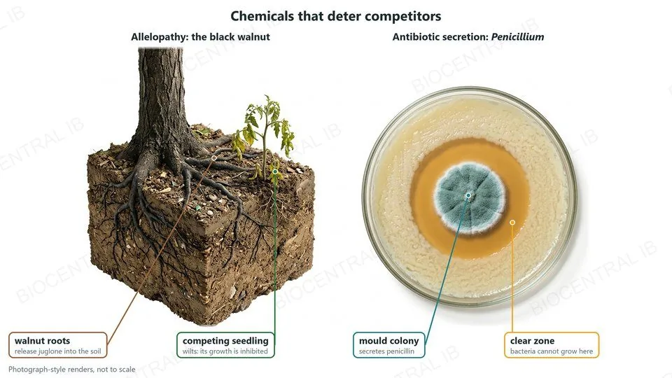
Allelopathy and antibiotic secretion are similar processes in which an organism releases a chemical substance into its environment to deter potential competitors.

Allelopathy is a plant releasing a chemical that inhibits the growth of nearby competing plants — the black walnut tree, which releases the compound juglone into the surrounding soil, is a well-documented example.
Antibiotic secretion is a microorganism releasing a chemical that kills or inhibits nearby competitors — the mould Penicillium secretes penicillin, which stops bacteria building their cell walls.
Both processes give the producing organism a competitive edge over neighbours without any direct physical contact or predation involved.

Why it mattersNaming one specific, real example of each process — not just describing the general concept — is what this statement requires.

Photograph-style renders: the roots of a black walnut tree release juglone into the soil, and a nearby competing seedling wilts, allelopathy; and a Penicillium mould colony on an agar plate secretes penicillin, leaving a clear zone where bacteria cannot grow

Where this shows up again

C1.3 · Photosynthesis

Energy for food chains originates from photosynthesis (C1.3). Explain why the efficiency of photosynthesis limits the total energy available to support higher trophic levels.

D3.3 · Homeostasis

Predator-prey cycles demonstrate negative feedback regulation in ecosystems. Compare this with negative feedback in blood glucose regulation (D3.3).

B4.2 · Ecological niches

Climate change alters the distribution of species. Using the niche concept (B4.2), explain why some species can shift their range while others face extinction.

C4.2 · Transfers of energy and matter

Carbon stored in fossil fuels was originally fixed by photosynthesis millions of years ago. Explain why burning fossil fuels represents a transfer of carbon from the long-term geological cycle to the short-term atmospheric cycle.

C4.1 Populations and communities — one-page recap

Screenshot this slide to revise from

Defining a population

Population: same species, interbreeding; separated by reproductive isolation, not just distance.
Sample rather than census — sampling must be random to avoid bias; some sampling error is unavoidable.

Measuring populations

Quadrats (sessile organisms) — small SD = evenly spread; large SD = patchy.
Lincoln index: population = (M × N) ÷ R, where N = total recaptured. Trap-shy → R low → overestimate; trap-happy → R high → underestimate.

Growth curves

Exponential (J-shaped, unlimited resources) tested by a straight line on a log-scale plot.
Sigmoid (S-shaped) plateaus at carrying capacity (K) — no lag phase in the idealised model.

Regulation & competition

Density-dependent factors (competition, predation, disease) push populations back to K by negative feedback.
Intraspecific relationships: competition or cooperation, within one species.

Interspecific relationships

Herbivory, predation, parasitism, pathogenicity (+/−: one gains, the other is harmed); interspecific competition (−/−).
Mutualism (both benefit): root nodules, mycorrhizae, zooxanthellae. Invasive species gain from "enemy release."

Testing & community control

Competition tested by lab experiment, field observation, or field manipulation; chi-squared tests species association.
Predator-prey cycles (lynx-hare): the predator peak lags the prey peak; communities show top-down or bottom-up control; allelopathy/antibiotics deter competitors chemically.

Next step

Now test yourself on C4.1

Reading the slides is half the job. The other half is answering questions the way the exam asks them.

54 quiz questions8 data questions5 exam questionsmarkschemes included

Practise C4.1 in the app → Try a free lesson

Unlock every lesson with Pro — quizzes, data questions and exam papers. Two lessons are completely free to try: A1.1 Water and B1.1 Carbohydrates and lipids.

One-page summary, key terms and sample questions for C4.1 →

A community is never just one story

From a single interbreeding population to a decade-long cycle between predator and prey, every relationship in this lesson is really one thing: a limit, and how life pushes against it.

C4.1 Populations and communities · BioCentral IB